
The Wise son:
As Wicked said in our previous post, ROC curve can help find the best cut-off point of a diagnostic test; a cut-off point which yields the best sensitivity (SE) and specificity (SP). Yet, since SE and SP have a ‘give and take’ relationship, how do we define “best”?
The Simple son:
Indeed, a compromise between SE and SP is required. Let’s recall the definitions:
Sensitivity - the ability to detect the ill people correctly (SE)
Specificity - the ability to detect the healthy people correctly (SP)
In some cases, SE is more important than SP, for example when a disease is highly infectious (and you all remember very well the COVID-19 tests..). In other cases, SP may be preferred over SE, say when the subsequent diagnostic testing is risky or costly. In such cases, a regulation agency may set the required minimal levels.
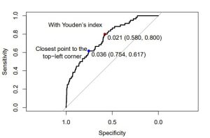
If there is no preference between SE and SP, a reasonable approach would be to maximize both indices, i.e.,
find the point on the ROC that maximizes SE+SP-1.
The Wicked son:
So, you mean to take the Youden’s index. Nah, I’ll take the point in which SP=SE. Wanna know why? Well, I can explain but I can’t promise you guys will understand. This point is mathematically the intersection of the line connecting the left-upper corner and the right-lower corner of the unit square and the ROC curve. This point of the curve is where the product of these two indices (SE x SP) is in its maximum.
I can give you one more method, just because I love to see my audience confused. You can also select the point on the ROC curve with the minimum distance from the left-upper corner of the unit square. Good luck to you all.
The Simple son:
Thank you, Wicked. You know that in a smooth curve, both methods will yield the same point.
But for the hack of it, I’ll show you these two methods on an empirical curve:
And this is the R code for that:
roc_cutpoint <- roc(grp ~ PS_2, data = Dat, auc=T, ci=T)
best1= pROC::coords(roc_cutpoint, "best",ret=c("t","sp","se"), transpose = T) #default method="youden"
best2= pROC::coords(roc_cutpoint,"best",ret=c("t","sp","se"), best.method = "closest.topleft", transpose = T) # method="closest.topleft"
plot(roc_cutpoint, print.thres="best", print.thres.best.method="youden")
points(best1[2],best1[3],pch=16,col="red")
plot(roc_cutpoint, print.thres="best", print.thres.best.method="closest.topleft",add=T)
points(best2[2],best2[3],pch=16,col="blue")
text(0.9,0.9,"With Youden’s index")
text(1.15,0.6,"Closest point to the\n top-left corner")
He who couldn’t ask:
Okay, okay, cut! you’ve made your point! All kinds of points! Is anybody in the mood for scotch on the ROCs? I need something strong after all your explanations.